Handling and visualising archive data from Strava
Some time last year, I deleted Strava. All I really cared about was how far I had ran, for how long, and where I had been. But you can get all of this information from open source alternatives like FitoTrack without handing over all your data to a commercial enterprise, or being bombarded with ads for a paid subscription. I’ve now settled with recording time for each run using my Casio, and then swiftly moving on with my life.
Before quitting Strava, I downloaded all my archived data. As much as I’d like to rise above obsessions over split times and average pace, I do like to look back on specific runs and check PBs periodically. When you archive Strava data, you get given your activities as individual GPX files. These files are of course pretty useless on their own, which I suppose deters many users from deleting the app. But with a fairly simple R script, you can get decent summaries of all your activities and mess around with data visualisation to your heart’s content. This is what I’ve begun to do myself, making all my data and code openly available.
The main challenge of the whole project was simply extracting the relevant information from the GPX files and compiling that information into a usable data frame. Printing the raw text contents of the files looks like absolute garbage, and without much experience of XML files, a lot my explorations were trial and error. I settled on using functions from the XML package to parse the files and extract information about each activity. This included stuff like the name (e.g., “Morning run”) and type (e.g., running, cycling), but importantly, also ping-level information collected throughout the duration of the activity, like the time of day, coordinate location and elevation at one or two second intervals.
The preliminary stuff at the top of script just loads in the packages required, lists all my GPX files in the data folder, and then imports them into RStudio using htmlTreeParse(). If you clone/download the repository and throw your GPX files into the data folder, you should be able to replicate everything shown here for your own data.
# Load libraries.
library(pbapply)
library(XML)
library(dplyr)
library(tidyr)
library(lubridate)
library(ggplot2)
library(leaflet)
library(maptiles)
library(tidyterra)
library(sf)

# Settings.
theme_set(theme_minimal())

# Create list of all the gpx files that we have.
file_names <- paste0(
  "data/",
  list.files("data", pattern = glob2rx("*.gpx"))
)

# Read them all into a list.
raw_list <- pblapply(file_names, function(x){
  htmlTreeParse(file = x, useInternalNodes = TRUE)
}
)
We can then execute the main parsing function: extracting the nodes we need and then sticking them together into a list of usable data frames. The final step uses st_as_sf() to convert the coordinates into an sf object, so we can easily calculate distances and create maps later on. I had around 200 activities and this took 1-2 monutes to run on a standard laptop.
# Function for extracting the relevant information.
acts_clean <- list()

for (i in seq_along(raw_list)){

# Extract name.
name <- xpathSApply(doc = raw_list[[i]], path = "//trk/name", fun = xmlValue)

# Extract type.
type <- xpathSApply(doc = raw_list[[i]], path = "//trk/type", fun = xmlValue)

# Extract coords.
coords <- xpathSApply(doc = raw_list[[i]], path = "//trkpt", fun = xmlAttrs)

# Extract elevation.
elevation <- xpathSApply(doc = raw_list[[i]], path = "//trkpt/ele", fun = xmlValue)

# Extract time.
time <- xpathSApply(doc = raw_list[[i]], path = "//trkpt/time", fun = xmlValue)

# Extract information into a dataframe.
gpx_sf <- data.frame(
  act_name    = name,
  act_type    = type,
  timestamps  = time,
  lat         = coords["lat", ],
  lon         = coords["lon", ],
  ele         = as.numeric(elevation)
) %>%
  mutate(timestamps = ymd_hms(timestamps),
         week_lub   = week(timestamps),
         year_lub   = year(timestamps)) %>%
  st_as_sf(coords = c(x = "lon", y = "lat"), crs = 4326)

# Insert each into the list.
acts_clean[[i]] <- gpx_sf

}
Each element of the acts_clean list is a single activity, with each row representing a single GPS ping recording the time and elevation.
We can easily bind all the data frames together. At this point, I subset my activities for running-only. You can of course keep all your different activity types, but remember that later on, you will need to group_by(act_type) to get equivalent summaries, or use some equivalent loop or facet.
# Bind together for broad summaries, then filter for runs only.
acts_sf <- bind_rows(acts_clean, .id = "act_id") %>%
  filter(act_type == "running")
The final key data handling step before we can begin summarising activities is spatial. At the moment, the ping-level data consists of coordinate locations recorded at one or two second intervals throughout the activity. But for mapping visuals and to easily calculate distances, we need to convert these series of points to lines. I do this by computing a union on each activity and casting the output to a linestring.
# Convert coords to lines.
acts_lines_sf <- acts_sf %>%
  group_by(act_id) %>%
  summarize(do_union=FALSE) %>%
  st_cast("LINESTRING") %>%
  ungroup()
We can then calculate the distance of each line using st_length(). I made this a standalone dataframe, with no spatial information, so it can be quickly joined back later on.
# Create df of the distances.
acts_dist_df <- acts_lines_sf %>%
  mutate(total_km = round(as.numeric(st_length(.)/1000), 2)) %>%
  as_tibble() %>%
  select(-geometry)
Okay, now we can actually calculate something… Here, we create usable ping-level information for each activity, including joining back the distance data.
# Ping-level data for every activity.
pings_df <- acts_sf %>%
  as_tibble() %>%
  group_by(act_id) %>%
  mutate(
  act_time   = max(timestamps)-min(timestamps),
  act_mins   = as.numeric(act_time, units = "mins"),
  ele_gain   = sum(diff(ele)[diff(ele) > 0])
) %>%
  ungroup() %>%
  left_join(acts_dist_df) %>%
  mutate(av_km_time = act_mins/total_km,
         act_id     = as.numeric(act_id),
         ping_id    = 1:nrow(.))
This allows us to make a usable descriptive summary table in one go.
# Summary table example.
sum_table_df <- pings_df %>%
  mutate(av_km_time = round(av_km_time, 2),
         act_mins   = round(act_mins, 2),
         ele_gain   = round(ele_gain, 0),
         act_date = format(date(timestamps), "%d.%m.%y")) %>%
  select(act_id, act_date, act_name, act_mins, total_km, ele_gain, av_km_time) %>%
  distinct(act_id, .keep_all = TRUE) %>%
  arrange(act_id)
This table pretty much contains most information I would ever want from my archive data. The script should be adaptable with your own data to add or remove anything.
| act_id | act_date | act_name | act_mins | total_km | ele_gain | av_km_time |
|---|---|---|---|---|---|---|
| 22 | 16.02.21 | Stretford - Jackson’s Boat - Home | 31.62 | 5.72 | 16 | 5.53 |
| 23 | 19.02.21 | Water Park - Jackson’s Boat - Home | 33.83 | 6.09 | 16 | 5.56 |
| 25 | 05.03.21 | Blair Witch Vibes | 28.70 | 5.33 | 18 | 5.38 |
| 26 | 10.03.21 | Stretford meander | 30.28 | 5.72 | 21 | 5.29 |
| 27 | 13.03.21 | Misjudged bridge situation | 35.18 | 6.74 | 25 | 5.22 |
| 29 | 20.03.21 | Charlie Don’t Surf | 34.23 | 6.21 | 17 | 5.51 |
| 32 | 24.03.21 | Final run | 55.65 | 10.04 | 25 | 5.54 |
| 33 | 30.03.21 | Jog back from test centre | 18.28 | 3.59 | 11 | 5.09 |
| 34 | 31.03.21 | Misjudged bridge situation 2 | 81.28 | 11.58 | 9 | 7.02 |
| 35 | 04.04.21 | Blimey | 38.70 | 7.81 | 23 | 4.96 |
| 36 | 10.04.21 | Morning run | 21.53 | 4.37 | 10 | 4.93 |
| 37 | 18.04.21 | First city run | 29.10 | 5.67 | 10 | 5.13 |
| 38 | 22.04.21 | Vondel run | 25.65 | 5.10 | 9 | 5.03 |
| 39 | 29.04.21 | Rembrandt run | 33.52 | 6.85 | 24 | 4.89 |
| 40 | 11.05.21 | Rembrandt run | 23.25 | 4.82 | 20 | 4.82 |
| 66 | 03.09.21 | Tide’s out legs out | 37.65 | 6.66 | 12 | 5.65 |
| 67 | 11.09.21 | Hilbre | 43.98 | 7.16 | 37 | 6.14 |
| 68 | 19.09.21 | Rembrandt run | 26.12 | 5.51 | 18 | 4.74 |
| 69 | 25.09.21 | Rembrandt run | 39.10 | 7.51 | 26 | 5.21 |
| 72 | 30.09.21 | Roman | 16.53 | 3.58 | 7 | 4.62 |
| 74 | 03.10.21 | PT | 20.52 | 3.43 | 12 | 5.98 |
| 75 | 04.10.21 | Night 5 | 24.23 | 5.05 | 12 | 4.80 |
| 76 | 08.10.21 | Following the lights | 24.43 | 5.15 | 16 | 4.74 |
| 77 | 09.10.21 | PT | 25.25 | 4.17 | 13 | 6.06 |
| 78 | 13.10.21 | Night 5 | 29.10 | 5.72 | 20 | 5.09 |
| 79 | 16.10.21 | Rembrandt run | 27.18 | 5.98 | 20 | 4.55 |
| 80 | 18.10.21 | PT | 32.12 | 5.07 | 19 | 6.33 |
| 81 | 21.10.21 | Evening 10 | 52.63 | 10.10 | 36 | 5.21 |
| 83 | 25.10.21 | PT | 30.67 | 5.06 | 19 | 6.06 |
| 84 | 27.10.21 | PT | 31.10 | 5.11 | 14 | 6.09 |
| 85 | 29.10.21 | Sloterplas 10 | 51.30 | 10.25 | 22 | 5.00 |
| 86 | 01.11.21 | Rembrandt run | 41.12 | 8.01 | 24 | 5.13 |
| 87 | 04.11.21 | PT | 28.37 | 5.06 | 17 | 5.61 |
| 88 | 06.11.21 | Porridge | 87.33 | 16.26 | 32 | 5.37 |
| 89 | 10.11.21 | Rembrandt recovery | 23.27 | 4.38 | 14 | 5.31 |
| 90 | 17.11.21 | Rembrandt run | 26.73 | 5.43 | 19 | 4.92 |
| 93 | 30.11.21 | Knee test | 30.93 | 5.94 | 17 | 5.21 |
| 94 | 09.12.21 | Kneed knees | 25.55 | 5.06 | 16 | 5.05 |
| 95 | 16.12.21 | Dune run | 30.78 | 5.52 | 10 | 5.58 |
| 96 | 24.12.21 | Explore | 29.60 | 3.92 | 108 | 7.55 |
| 97 | 26.12.21 | Hill climber | 28.97 | 5.09 | 156 | 5.69 |
| 98 | 28.12.21 | Explore turbo | 22.70 | 3.94 | 111 | 5.76 |
| 99 | 02.01.22 | PT | 20.13 | 3.46 | 12 | 5.82 |
| 100 | 05.01.22 | Rembrandt run | 26.92 | 5.21 | 18 | 5.17 |
| 101 | 09.01.22 | Combo | 47.17 | 8.95 | 21 | 5.27 |
| 102 | 16.01.22 | Sloterplas 10 | 53.55 | 10.19 | 23 | 5.26 |
| 103 | 20.01.22 | Night run | 27.38 | 5.12 | 16 | 5.35 |
| 104 | 22.01.22 | Rembrandt run | 24.73 | 5.25 | 19 | 4.71 |
| 105 | 26.01.22 | Evening run | 26.87 | 5.25 | 18 | 5.12 |
| 106 | 29.01.22 | Sloterplas 10 | 50.10 | 10.16 | 32 | 4.93 |
| 107 | 03.02.22 | Evening run | 25.07 | 5.11 | 15 | 4.91 |
| 108 | 06.02.22 | Rembrandt run | 24.77 | 5.04 | 19 | 4.91 |
| 109 | 08.02.22 | West run | 40.47 | 8.08 | 27 | 5.01 |
| 110 | 12.02.22 | West 10 | 53.22 | 10.48 | 29 | 5.08 |
| 111 | 15.02.22 | Rembrandt run | 22.57 | 5.03 | 18 | 4.49 |
| 112 | 23.02.22 | Lunchtime run | 16.00 | 3.22 | 11 | 4.97 |
| 113 | 25.02.22 | Morning run | 24.75 | 5.14 | 21 | 4.82 |
| 115 | 28.02.22 | West run | 41.42 | 8.03 | 27 | 5.16 |
| 116 | 01.03.22 | Lunchtime run | 14.05 | 3.00 | 10 | 4.68 |
| 117 | 12.03.22 | Spring | 25.32 | 5.16 | 19 | 4.91 |
| 119 | 16.03.22 | Sandy | 24.68 | 5.03 | 18 | 4.91 |
| 120 | 19.03.22 | Rembrandt run | 40.48 | 7.78 | 27 | 5.20 |
| 121 | 21.03.22 | Morning run | 15.33 | 2.85 | 9 | 5.38 |
| 124 | 27.03.22 | Evening run | 16.43 | 3.02 | 9 | 5.44 |
| 125 | 06.04.22 | Back to it | 33.18 | 6.40 | 19 | 5.18 |
| 126 | 15.04.22 | Afternoon run | 12.15 | 2.27 | 7 | 5.35 |
| 128 | 18.04.22 | Sloterplas 10 | 51.45 | 10.19 | 27 | 5.05 |
| 129 | 20.04.22 | Cake | 36.10 | 7.09 | 20 | 5.09 |
| 130 | 27.04.22 | Rembrandt run | 25.22 | 5.02 | 18 | 5.02 |
| 134 | 08.05.22 | Sunday run | 20.52 | 4.02 | 14 | 5.10 |
| 135 | 09.05.22 | Morning run | 12.73 | 2.55 | 9 | 4.99 |
| 136 | 14.05.22 | West meander | 29.15 | 5.80 | 16 | 5.03 |
| 138 | 16.05.22 | PT | 13.20 | 2.36 | 7 | 5.59 |
| 139 | 20.05.22 | Run | 12.77 | 2.63 | 9 | 4.85 |
| 140 | 21.05.22 | Sloterplas 10 | 53.88 | 10.08 | 23 | 5.35 |
| 141 | 25.05.22 | Rembrandt run | 27.37 | 5.01 | 18 | 5.46 |
| 143 | 29.05.22 | Rembrandt run | 25.25 | 5.25 | 18 | 4.81 |
| 144 | 04.06.22 | West | 35.17 | 7.12 | 17 | 4.94 |
| 145 | 12.06.22 | Rembrandt run | 21.60 | 4.51 | 15 | 4.79 |
| 147 | 10.07.22 | Urban trail series | 36.95 | 6.45 | 23 | 5.73 |
| 148 | 27.07.22 | Heal the heel | 17.55 | 3.40 | 11 | 5.16 |
| 150 | 01.08.22 | Rembrandt run | 24.92 | 4.34 | 14 | 5.74 |
| 151 | 05.08.22 | Alright then | 24.47 | 5.04 | 16 | 4.85 |
| 152 | 10.08.22 | Toasty | 30.18 | 6.03 | 16 | 5.01 |
| 153 | 14.08.22 | West | 37.05 | 7.22 | 20 | 5.13 |
| 154 | 19.08.22 | Westish | 25.50 | 5.44 | 14 | 4.69 |
| 155 | 22.08.22 | Blimey | 26.57 | 5.13 | 129 | 5.18 |
| 156 | 26.08.22 | Jogaroo | 15.70 | 3.47 | 13 | 4.52 |
| 157 | 01.09.22 | West 10 | 48.28 | 10.12 | 27 | 4.77 |
| 158 | 11.09.22 | Pancakes | 63.33 | 12.86 | 32 | 4.92 |
| 159 | 18.09.22 | Summit attempt | 26.00 | 4.16 | 116 | 6.25 |
| 160 | 25.09.22 | Paros 5 | 33.90 | 5.79 | 163 | 5.85 |
| 161 | 29.09.22 | West (pt1) | 8.08 | 1.64 | 4 | 4.93 |
| 162 | 29.09.22 | West (pt2) | 35.65 | 7.37 | 18 | 4.84 |
| 163 | 03.10.22 | Rembrandt run | 22.20 | 4.62 | 17 | 4.81 |
| 164 | 06.10.22 | West | 43.18 | 8.22 | 31 | 5.25 |
| 165 | 08.10.22 | Ginger cake | 85.43 | 16.56 | 47 | 5.16 |
| 166 | 13.10.22 | Rembrandt run | 21.02 | 4.34 | 15 | 4.84 |
| 167 | 16.10.22 | Amsterdam half | 106.42 | 21.98 | 70 | 4.84 |
| 168 | 30.10.22 | Rembrandt run | 22.60 | 4.46 | 16 | 5.07 |
| 169 | 02.11.22 | West | 37.88 | 7.81 | 24 | 4.85 |
| 170 | 05.11.22 | Rembrandt run | 24.57 | 5.11 | 20 | 4.81 |
| 171 | 09.11.22 | West | 31.20 | 7.24 | 25 | 4.31 |
| 172 | 11.11.22 | Rembrandt run | 22.20 | 4.48 | 17 | 4.96 |
| 173 | 15.11.22 | West | 28.17 | 6.09 | 17 | 4.63 |
| 174 | 15.11.22 | West finish | 5.15 | 1.11 | 5 | 4.64 |
| 175 | 19.11.22 | West | 31.87 | 7.06 | 19 | 4.51 |
| 176 | 22.11.22 | PT | 40.63 | 7.06 | 25 | 5.76 |
| 177 | 24.11.22 | Rembrandt run | 31.65 | 5.88 | 20 | 5.38 |
| 178 | 27.11.22 | West 10ish | 56.10 | 11.23 | 39 | 5.00 |
| 179 | 03.12.22 | West 10ish | 50.78 | 10.92 | 29 | 4.65 |
| 180 | 06.12.22 | West meander | 29.72 | 6.18 | 21 | 4.81 |
| 181 | 08.12.22 | West / Sloterplas | 38.80 | 8.22 | 25 | 4.72 |
| 182 | 13.12.22 | Canal loop | 28.10 | 5.71 | 19 | 4.92 |
| 183 | 17.12.22 | West / Sloterplas | 53.48 | 10.98 | 32 | 4.87 |
| 184 | 23.12.22 | Wirral | 82.30 | 15.64 | 33 | 5.26 |
| 185 | 28.12.22 | Windy bastard | 23.65 | 4.67 | 152 | 5.06 |
| 186 | 30.12.22 | LPA (pt1) | 7.35 | 1.33 | 45 | 5.53 |
| 187 | 30.12.22 | LPA (pt2) | 49.72 | 9.77 | 139 | 5.09 |
| 188 | 04.01.23 | Rembrandt run | 21.73 | 4.74 | 18 | 4.59 |
| 189 | 08.01.23 | Egmond half | 113.02 | 21.85 | 89 | 5.17 |
| 190 | 18.01.23 | Back to it | 16.02 | 3.44 | 11 | 4.66 |
| 191 | 22.01.23 | Rembrandt run | 28.62 | 4.75 | 16 | 6.02 |
| 194 | 04.02.23 | Rembrandt run | 16.45 | 3.99 | 15 | 4.12 |
| 195 | 05.02.23 | PT | 40.65 | 7.38 | 27 | 5.51 |
| 196 | 08.02.23 | Rembrandt run | 18.65 | 4.23 | 13 | 4.41 |
| 197 | 12.02.23 | Rembrandt run | 12.08 | 2.95 | 11 | 4.10 |
| 198 | 07.03.23 | Rembrandt run return | 17.60 | 3.92 | 16 | 4.49 |
| 199 | 11.03.23 | Rembrandt run | 29.93 | 6.36 | 20 | 4.71 |
| 200 | 16.03.23 | Westish | 25.85 | 5.87 | 16 | 4.40 |
| 201 | 19.03.23 | Urban pickle trail series | 101.98 | 14.03 | 41 | 7.27 |
| 202 | 23.03.23 | Bats | 14.32 | 2.38 | 8 | 6.02 |
| 203 | 26.03.23 | Zandvoort | 72.52 | 12.35 | 102 | 5.87 |
| 204 | 24.07.23 | Chart | 18.23 | 3.16 | 38 | 5.77 |
| 205 | 24.07.23 | Chart 2 | 4.78 | 0.85 | 12 | 5.63 |
| 207 | 03.10.23 | Come on, legs | 15.75 | 2.85 | 10 | 5.53 |
| 208 | 07.10.23 | Michael Ketone | 16.98 | 3.02 | 10 | 5.62 |
| 1 | 16.10.23 | Jacket | 24.25 | 4.31 | 15 | 5.63 |
| 2 | 17.10.23 | PT | 14.43 | 2.20 | 7 | 6.56 |
| 3 | 21.10.23 | Bugger this | 15.73 | 3.02 | 10 | 5.21 |
| 4 | 25.10.23 | The Heel Strike’s Back | 20.13 | 4.10 | 14 | 4.91 |
| 5 | 30.10.23 | Rembrandt run | 21.63 | 4.32 | 15 | 5.01 |
| 6 | 04.11.23 | 21 bathrooms | 27.33 | 4.56 | 15 | 5.99 |
| 7 | 25.11.23 | Room for a small one | 10.87 | 2.10 | 8 | 5.17 |
| 8 | 29.11.23 | Lil one | 11.18 | 1.77 | 7 | 6.32 |
| 9 | 24.12.23 | Sherry | 15.85 | 2.50 | 88 | 6.34 |
| 10 | 27.12.23 | Audacity | 30.80 | 4.75 | 50 | 6.48 |
| 11 | 30.12.23 | Beachy | 10.27 | 2.01 | 6 | 5.11 |
| 12 | 02.01.24 | Watery bastard | 26.77 | 4.79 | 11 | 5.59 |
| 13 | 04.01.24 | Mr. Motivator | 12.70 | 2.65 | 10 | 4.79 |
| 14 | 06.01.24 | Jumbo | 15.60 | 2.44 | 9 | 6.39 |
| 15 | 10.01.24 | Nippy | 12.52 | 2.61 | 9 | 4.80 |
| 16 | 14.01.24 | No Vondelling | 25.70 | 5.13 | 15 | 5.01 |
| 17 | 18.01.24 | Cheese | 25.58 | 4.38 | 17 | 5.84 |
| 18 | 22.01.24 | Kattenlaan | 21.25 | 4.23 | 12 | 5.02 |
| 19 | 24.01.24 | Vondel thingy | 24.72 | 5.08 | 14 | 4.87 |
| 20 | 27.01.24 | Strava are bastards. Moving to FitoTrack | 15.28 | 2.76 | 9 | 5.54 |
That said, the table is quite boring. The fun derived from going through GPX file hell is in the visualisation that follows. I haven’t spent too long on this yet, so there’s plenty more fun to be had. Before getting into the ggplot2 chunks, I tidy up the summary table by renaming some columns and pivoting everything to long format. The pivot makes visualisation much easier later on.
# Initial handling before visuals.
sum_visuals_df <- sum_table_df %>%
select(-act_date, -act_name) %>%
rename(`Time (mins)` = act_mins,
`Distance (km)` = total_km,
`Elevation gain (metres)` = ele_gain,
`Km pace (mins)` = av_km_time) %>%
pivot_longer(cols = -act_id,
names_to = "measure",
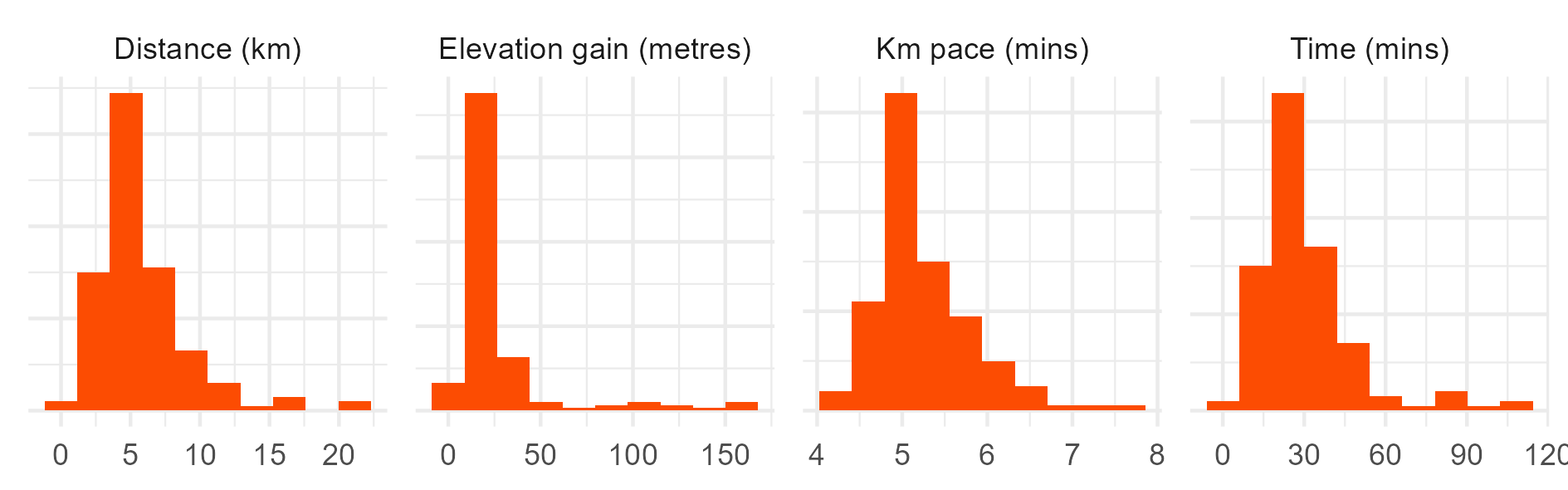
values_to = "value")Now we can easily create some visual summaries of distributions across different metrics.
# Histograms.
ggplot(data = sum_visuals_df) +
  geom_histogram(mapping = aes(x = value), bins = 20, fill = "#fc4c02") +
  facet_wrap(~measure, scales = "free", ncol = 4) +
  labs(y = NULL, x = NULL) +
  theme(
    axis.text.y = element_blank()
  )
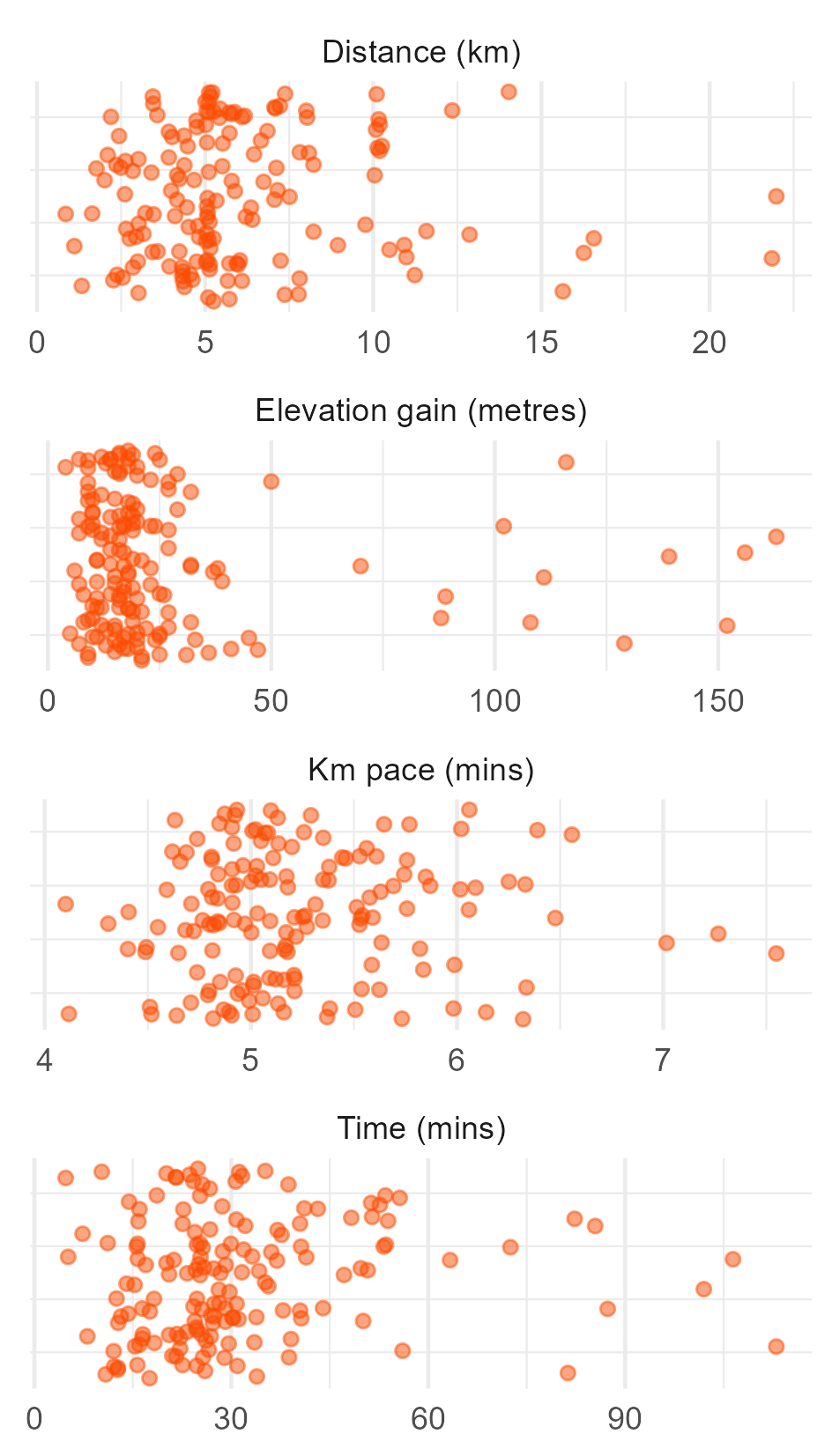
Or plot the individual points.
# Scatter plot of individual runs.
ggplot(data = sum_visuals_df) +
  geom_jitter(mapping = aes(x = value, y = 0),
               colour = "#fc4c02", alpha = 0.5) +
  facet_wrap(~measure, scales = "free", nrow = 4) +
  labs(y = NULL, x = NULL) +
  theme(
    axis.text.y = element_blank(),
    panel.grid.major.y = element_blank()
  )
We can also select individual runs to visualise things like elevation. Here, I choose a run manually by name because it was a good example of a hilly one. Be careful doing this if you tend to use the same name for different runs. You can always use the activity id numeric variable instead.
# elevation.
pings_df %>%
  filter(act_name == "Hill climber ") %>% # Name has to be distinct!
  ggplot(data = .) +
  geom_ribbon(mapping = aes(x = ping_id, ymin = min(ele)*0.5, ymax = ele, group = 1),
              fill = "#fc4c02", linewidth = 1) +
  theme_minimal() +
  theme(
    axis.text.x = element_blank()
  ) +
  labs(y = "Elevation (metres)", x = NULL)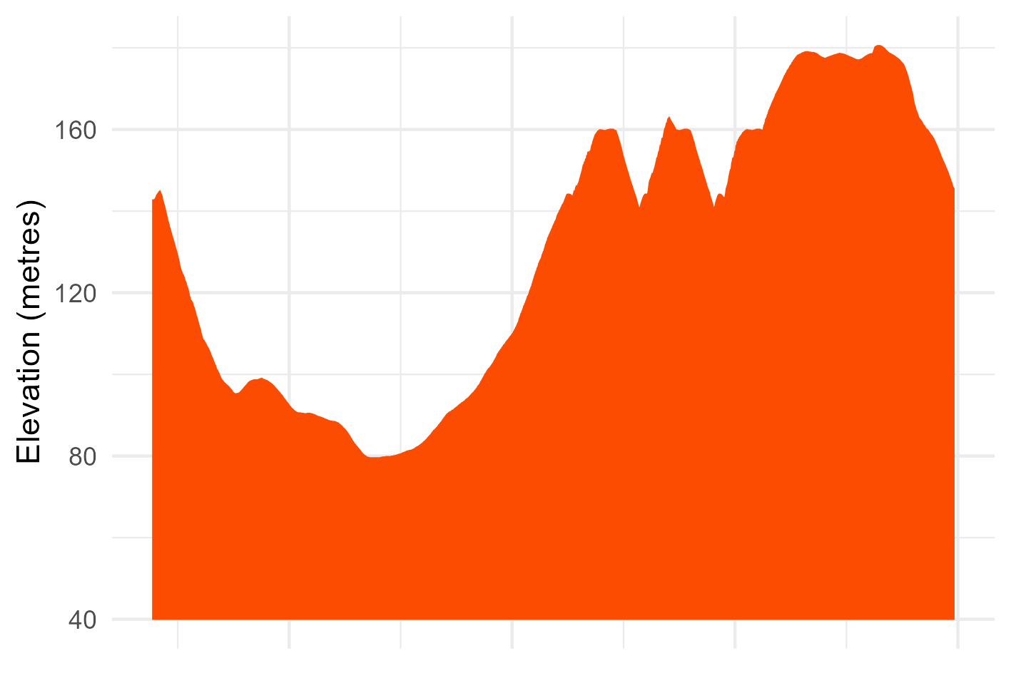
To make some decent maps, we need to convert the point-level pings to lines. I do this for every activity in one go using group_by(), followed by a spatial union and then ensuring the output is treated as a line.
# Single activity map.
# First, create the linestrings from the points.
acts_line_sf <- acts_sf %>%
  group_by(act_id) %>%
  summarize(do_union=FALSE) %>%
  st_cast("LINESTRING") %>%
  ungroup()
While not necessary, to give our activity maps some geographic context, I obtain CARTO base maps for each activity. You could do this for every activity in one go, but for now I just do it for a single example.
# Single activity selection for examples.
act_i <- 1

# Second, obtain the osm layer for a single activity.
osm_posit <- get_tiles(
  filter(acts_line_sf, act_id == act_i),
  provider = "CartoDB.Positron",
  crop = FALSE, zoom = 15
  )
Then we can get mapping. I do a small wrangle beforehand, first to subset the lines for my example activity, and then to join back the activity information. The latter step means I can make a joint graphic of both the map and the activity information (e.g., distance, pace) at some point later on, if wanted.
# First we subset to get the label and keep the other data.
act1_sf <- acts_line_sf %>%
  filter(act_id == act_i) %>%
  mutate(act_id = as.numeric(act_id)) %>%
  left_join(sum_table_df, by = "act_id") # get info back.

# Map it out.
ggplot(data = act1_sf) +
  geom_spatraster_rgb(data = osm_posit) +
  geom_sf(colour = "#fc4c02", linewidth = 1) +
  theme_void()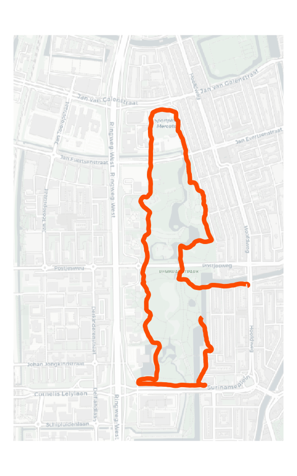
We can also, with a little effort, create an interactive map using leaflet. Here, I just use the basic Open Street Map layer, but you can add other (prettier) layers and an interactive legend with a bit more fiddling. You can view a more elaborate example here.
# Interactive map for single activity.
leaflet() %>%
  addTiles() %>%
  addPolylines(data = act1_sf,
               color = "#fc4c02")
For now, that’s that! Please feel free to make use of the code for your own archived data, and if you have any suggestions or make any further progress, feel free to get in touch.
Samuel Langton
I am currently a Lecturer in Quantitative Criminology at the University of Manchester. I have previously worked as a postdoc at the NSCR and a research software consultant at Amsterdam UMC.