Misrepresentation in maps: mini-survey results from the Ministry of Defence

Background

Thanks to various pieces of clever research and fantastic books, we know that people can misinterpret data visualisations. Maps are no different. One reason why people can misinterpret maps is due to the size of the areas being visualised. Never have I seen more spatial visualisations flying around than during the COVID-19 pandemic: people were desperate to compare how different countries, regions or neighbourhoods were fairing, and maps are an accessible and beautiful way to convey this information. But, countries, regions and neighbourhoods can vary considerably in size. Take this map of England below. It was published by Public Health England and subsequently reported by the BBC in November 2020. It shows the different lockdown tiers which were set to come into place before Christmas that year.

The problem with maps like this is that the areas being mapped (local authorities) are not uniform in size or shape. Densely populated local authorities, such as those that comprise London, are almost invisible, while less urbanised areas, which are geographically large, dominate the visual. It’s a rare occasion where London not being the focus of attention is probably not a good thing, considering the number of people residing in these lockdown tiers. The makers of the map were probably well-intentioned: after all, they are using the real, raw boundaries of local authorities – but that doesn’t guarantee that the map will convey the underlying data clearly. In this particular case, it is reasonably likely that there isn’t much variation going on between these small, compact units – but of course, we cannot be certain by examining this map in isolation, and let’s be honest, not everyone is going to read the text accompanying a beautiful map.

Alternative mapping methods

While the government and media reporting of the pandemic gave us plenty of the above mapping examples, the issue is by no means uncommon, or particularly new. Just a few years earlier, maps were widely used to report on the result of the EU referendum in the UK (e.g. BBC). Largely due to the different voting behaviour between densely populated, urban London and the rest of the country, maps which visualised the result using raw local authority boundaries could be highly misleading. Geographically vast, leave-voting areas dominate the map, rendering the remain-strong London almost invisible. This also makes it more difficult for people to spot spatial patterns, such as like-for-like areas being geographically proximal to one another.

This is where alternative forms of map can be useful. By deliberately distorting raw boundaries, or by assigning geographic areas to uniform shapes, we can actually improve the accuracy with which people interpret the data underlying a map. Back in 2019, in a paper together with Reka, we examined whether alternative types of map could more accurately convey the clustering of EU referendum remain voters in London compared to the original local authority boundaries (a pre-print of this paper is also freely available here). We did this using a sample of ~800 Reddit users. We found that people were more likely to interpret information about the geographic patterning of the referendum result accurately when looking at two alternative types of map, balanced cartograms and hexograms, compared to the raw boundaries. But, other alternatives (hex and square grids) made people less likely to accurately interpret the same information, compared to the raw boundaries. So, not all alternatives worked, but our findings made it clear that (1) mapping raw boundaries can be an inappropriate way of conveying spatial information, and (2) alternative mapping methods can (but not always) convey geographic clustering better than raw boundaries. There were of course caveats to our study (e.g., generalisability), so we’d encourage you to read the full thing too!

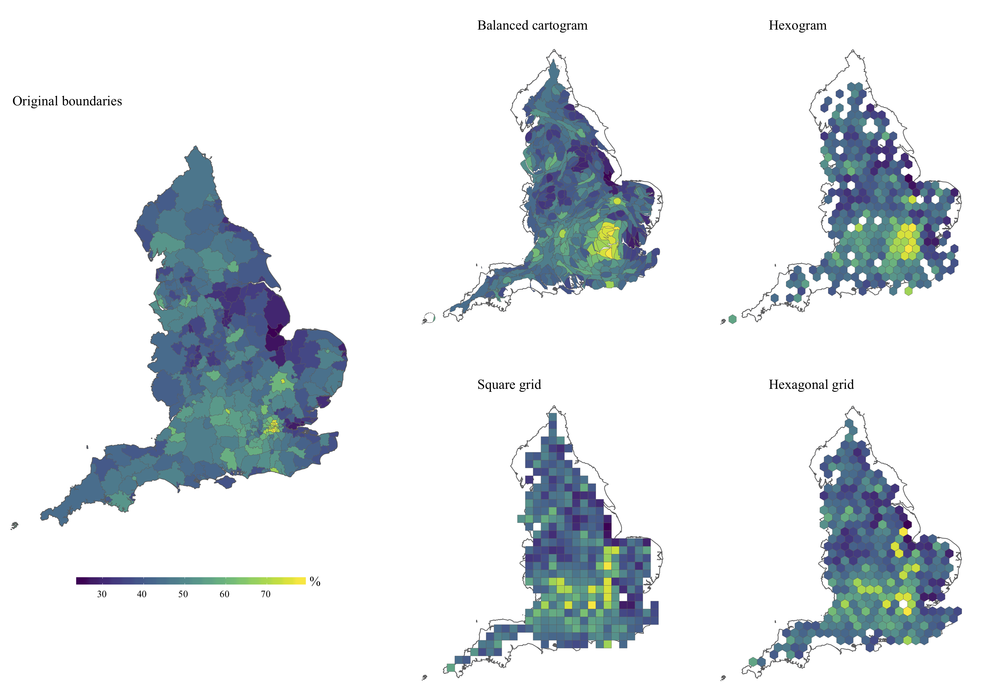
Figure 1: Proportion of remain voters in England at the local authority level, visualised using different mapping techniques. Source: Langton & Solymosi (2019).

MOD extension

Following our study, and an awesome training video that Reka made in collaboration with SAGE, we were contacted by a scientific adviser at the UK’s Ministry of Defence to share our musings and findings on this topic to MOD personnel. While we didn’t know the precise role and background of the attendees, we knew that many had a military background, and had expertise in analytics and scientific research. You can find the slides for this on Reka’s website. We took this opportunity to conduct another mini-survey using different data, with a slightly different focus, and of course, a very different sample of respondents.

Data

The broad motivation behind the mini-survey was comparable: Do people make worse estimates about the underlying data when observing the original boundaries of a map, in comparison to alternative methods (e.g. hex maps)? To study this, we took the example of neighbourhood deprivation in England. This is a salient example of the issue associated with mapping small areas. Neighbourhoods in England–defined as Lower Super Output Areas–are designed to be uniform by population size (~1500 residents). But, deprived areas are much more likely to be densely populated, and thus geographically small, compared to wealthier neighbourhoods, which are often sparsely populated and therefore geographically large. As a result, even regions containing lots of deprived neighbourhoods might not, at first glance and with limited information, appear particularly deprived.

Based on our previous study, we boldly thought: hey, using alternative mapping techniques we can better convey the underlying data compared to the original neighbourhood boundaries. To test this, we obtained data on neighbourhood deprivation across three local authorities: Birmingham, Hartelpool and Burnley. As measured using the Index of Multiple Deprivation in 2019, these are some of the most deprived local authorities in England. For each region, we mapped out neighbourhood deprivation using three different mapping techniques: the raw boundaries, a hex grid (using the geogrid R package) and a dorling cartogram (using the cartogram package) scaled by resident population. Here’s Birmingham using these techniques. For simplification, we recoded the typical IMD score which runs from 1 (most deprived) to 10 (least deprived) to 1-5 (e.g., 1 and 2 were recorded to 1, and so on).

Nine maps (three regions, each visualised three different ways) were shown to the MOD participants one after the other. To try and mitigate against respondents using the previous answer as a guide, the same regions were never shown consecutively. For each map, respondents were asked to estimate the percentage of residents living in the most deprived neighbourhood (1 - dark blue). Of course, we knew the answer to this already, because we had the underlying data, but the respondents were asked to make this assessment with limited information. So, for each map, we would end up with a range of different estimates from respondents, which could then be compared to the true figure. The larger the degree of error between the estimates and the true number, the ‘worse’ the map was communicating the underlying data.

Here, it’s worth noting that when we were discussing the survey findings during the MOD presentation, after it had been completed, a number of respondents questioned whether the colour of the first category was ‘dark blue’, but rather, a shade of purple. We return to this later. Aside from making me question my ability to distinguish different shades of blue-purple, it brought up another interesting discussion about visualisation and surveys more generally. We’ve shared a screenshot of the first page of the survey below.

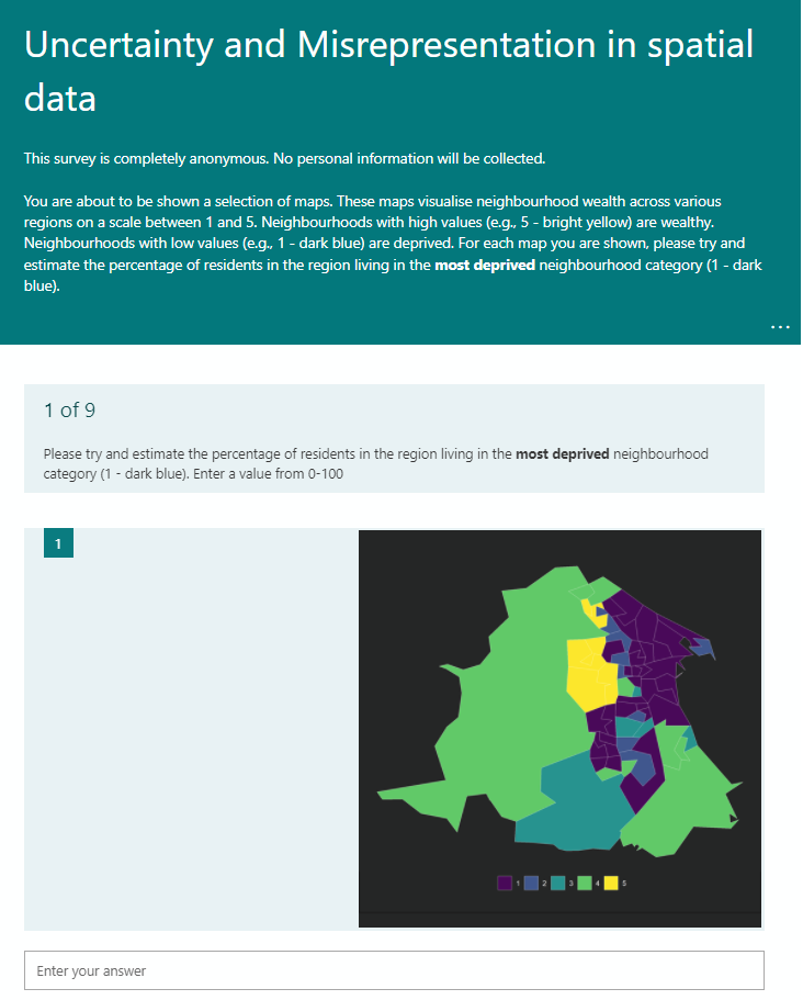
Figure 2: A screenshot from the first page of the survey. The survey was created is MS Forms.

Results

Respondents had around 24 hours to complete the survey. In total, we had 70 responses.¹ Two respondents were dropped because they were tests. Two additional people were dropped for missing questions, and two more were dropped because they contained text answers. This gave us 64 completed surveys for analyses. You can re-create all the maps and analyses reported here using the code on the corresponding GitHub repository.

In the graphic below, we plot the distribution of respondents’ estimates for each region, and each map type. The dotted line represents the true value (reality). Of course, this true value is identical for each region, irrespective of the map type. A number of things emerge from this visual. Let’s start with the distribution of estimates when people were observing the original boundaries. In all three study regions, people tended to underestimate the percentage of residents living in the most deprived category. This is exactly what we would expect: the most deprived neighbourhoods are geographically small, occupying a smaller proportion of the map, so with no other information available, people underestimate.

Hex maps, on the other hand, which assign each neighbourhood polygon to a grid of hexagons, appear to improve the accuracy of people’s estimates. Generally speaking, respondents got closer to the true figure when viewing the hex map compared to the original boundaries. Particularly with Burnley and Hartlepool, there is a noticeable peak in the distribution close to the true value. This is quite expected: the hexagons, which are uniformly sized and shaped, reflect the similarly uniform residential size of neighbourhoods. In this way, they are quite similar to waffle charts but arranged to reflect the geography of the study region. That said, we know from our previous study using the EU referendum data, and a visual inspection of the maps used here, that hex grids can massively distort the spatial distribution of polygons. So, while the hex maps used here have some clear benefits when it comes to interpreting aggregate information, the spatial patterning itself might be lost along the way. Interestingly, there is no such peak in respondent estimates around the true figure for the Birmingham hex map. This might be a result of the sheer number of neighbourhoods compared to Burnley and Hartlepool, or because there was less variation in the size of neighbourhoods nested within the city

When observing the dorling maps, people often slightly overestimated the percentage of people residing in the most deprived neighbourhood. It’s not immediately clear why this is the case (at least, not to me), but this overestimation was pretty common across all three regions. Even though Lower Super Output Areas are designed to be fairly similar in residential size, there is still some variability, which is reflected in the differently sized circles representing each neighbourhood. Interestingly, this was the only map type which actually conveyed data about residential size. But, without any additional information or clarification (e.g., an extra legend), the dorling maps appear to have misled respondents fairly consistently across regions.

The plot below visualises the same data slightly differently. Here, we plot the difference between each respondents’ estimate and the true figure, jittered slightly along the y-axis to avoid overlap between points. A boxplot summarises the overall spread. This does a reasonable job at demonstrating the degree of error in respondents’ estimates. But, it also shows the considerable spread in responses – making this estimate is not easy, and respondents clearly sometimes make completely erroneous guesses, possibly due to the survey design. In this particular case, the spread is minimised (overall) when using hex maps with a relatively small number of areas, as is the case with Hartlepool and Burnley.

Discussion

The findings from our mini-survey of MOD participants raise a number of interesting points – but also plenty of further questions. First, we found pretty good evidence to suggest that, in the absence of detailed information, visualising raw boundaries can misrepresent the data underlying a map. Here, respondents tended to underestimate the proportion of residents living in highly deprived neighbourhoods when observing a map of the raw boundaries. This is precisely what we would expect due to their small geographic size in comparison to wealthier neighbourhoods. Instead, by assigning neighbourhoods to a hex grid, which are uniform in size and shape, respondents were able to make fairly accurate estimates. But, this benefit comes at a cost, namely, the distortion of spatial patterning. The dorling cartogram introduced the opposite effect as the original boundaries, with people tending to slightly overestimate the overall proportion. So, alternative methods are not always ‘better’ but are certainly worth considering. Ultimately, it just depends on the aim of the research, and the message you want to convey with the visualisation.

Conducting the mini-survey itself brought up an interesting learning point on survey design for these kinds of questions. As we noted earlier, many respondents questioned the description of the ‘most deprived’ category as ‘dark blue’. We used a colourblind friendly palette (viridis), but clearly, referring to colours by name in isolation is problematic. Different people will interpret the same colours differently, even with colourblind friendly palettes like viridis. You can try this out for yourself online using the viridis documentation. Fortunately, because we referred to the category by both colour and number, I think we largely avoided total confusion, otherwise we’d expect a clear bi-modal distribution in answers, or many ‘zero’ answers. Nevertheless, for a full-scale survey with a robust design and a generalisable sample, we would want to pilot the survey thoroughly beforehand to weed-out issues like this early on.

Speaking of full-scale surveys: of course, mini-surveys like this are fun and interesting, and as noted, make useful learning experiences, but there is a huge ‘generalisability’ question over the results. We don’t know much about our MOD sample, so we cannot even generalise to the organisation itself. Any future work which aspires to generalisation might want to consider what populations are interesting and useful, and which map types (and for what purposes) are most relevant for that population. If anyone has pointers, suggestions or feedback, please do get in touch!